pgvector vs Qdrant vs Weaviate at 10k: No Cliff

I was going to write a shootout. Three vector databases, ten thousand agent memories, ten thousand ways to look clever. Load the same corpus into pgvector, Qdrant, and Weaviate, run the same queries, publish a winner.

I got as far as pgvector, watched every filtered query return in under two milliseconds, and stopped. The cliff I was going to warn everyone about did not exist at this scale, and I refuse to pretend it did.

This is what I actually measured, what the published benchmarks say for the scales I did not measure, and where the crossover between these three engines actually lives — as of pgvector 0.8.6 (July 2026), Qdrant 1.19 (August 2026), and Weaviate 1.39 (August 2026).

pgvector vs Qdrant vs Weaviate: what each engine is actually best at

The setup, and what makes it honest

I ran pgvector 0.8.6 on Postgres 17 in a fresh Docker container on my laptop. I loaded 10,000 rows into a memories table with one 1536-dim vector column, plus agent_id (1–3), project_id (1–20), and created_at. HNSW index with defaults (m=16, ef_construction=64), plus btrees on project_id and (agent_id, created_at). Two hundred queries per condition, warm cache.

The vectors are random Gaussian noise. That matters for recall quality — random vectors cluster inside a hypersphere shell and are unrealistically friendly to nearest-neighbor search — but for measuring the mechanism of filter-vs-index interaction, they are exactly the right control. If the filter path is broken, random data will not save it.

Two things I did not measure and will not fabricate: Qdrant and Weaviate at the same 10k. Running three engines with three configurations, warming three caches, and defending three sets of tuning choices is a project, not a blog post. Their own benchmark exists and I would rather cite it than approximate it.

What pgvector actually did

Three query shapes, all LIMIT 10, cosine distance. Numbers are from the script I linked at the bottom.

Query	p50	p95	p99
unfiltered top-10	1.31 ms	1.67 ms	1.88 ms
`WHERE project_id = ?` (≈ 500 candidates)	1.88 ms	3.20 ms	3.48 ms
`WHERE agent_id = ? AND created_at > NOW() - 1 min`	1.39 ms	2.53 ms	3.82 ms

The story I had prepared, based on tweets I had read, went: WHERE project_id = ? would blow up because HNSW does not know about the filter, so the graph traversal wanders forever hunting for ten survivors. That story reproduces at a million vectors with hnsw.ef_search=40 and a filter that leaves the walk starving. It does not reproduce at ten thousand rows with a 1-in-20 filter, because there are 500 candidates and HNSW finds ten of them without breaking a sweat.

I also enabled hnsw.iterative_scan = strict_order, which pgvector 0.8.0 added for exactly this case (pgvector README on iterative index scans). The project_id p50 dropped from 1.88 ms to 1.72 ms. That is noise, not a fix, because there was nothing to fix — every default-HNSW query already returned all ten requested rows. I counted, thirty times, both with and without iterative_scan. Ten for ten.

That is the finding I would have missed if I had trusted the shootout draft: at agent-memory scale, the pgvector filter cliff is a myth. Everything runs in single-digit milliseconds and the tuning knob most people cite does not activate.

Where the crossover actually lives

Qdrant’s own benchmark (qdrant.tech/benchmarks) uses dbpedia-openai-1M-angular — one million vectors at 1536 dims — and that is where the filter path becomes the thing that separates engines. The graph is deeper, ef_search matters, and post-filter either misses recall or spends much more traversal to hit k=10. Their write-up on filtered search names three failure modes: speedup when a payload index helps, slowdown when the filter is a burden the index cannot serve, and recall collapse for engines that filter after the graph has already emitted. Their benchmark repo at github.com/qdrant/vector-db-benchmark is runnable — I did not run it, because reproducing three engines at 1M is a week, and the results already exist.

The public ann-benchmarks project (ann-benchmarks.com) is the other credible source. It tests HNSW variants, Qdrant, Weaviate, and dozens of libraries on small datasets like glove-100 and gist-960 — good for algorithm-level comparisons, silent on filtered search at production scale. If you are picking a vector store for an agent that filters by tenant, ann-benchmarks will not answer you.

The honest position: my 10k test says pgvector is fine here. The published 1M-with-filters test says Qdrant leads on that specific axis. Nobody I trust has published a rigorous 3-way filtered benchmark for the middle range, and I am not going to invent one. If you have followed my post on three sub-agents reviewing the same PR, you know the pattern: it is not the average case that separates good from bad, it is the case nobody planned for.

What each cloud actually charges (August 2026)

I opened three pricing pages this morning:

Deployment	Public price	Source
Supabase Pro (pgvector on managed Postgres)	$25/mo base, includes Micro compute (2-core ARM / 1 GB); $0.125/GB disk >8 GB; $0.09/GB egress >250 GB	supabase.com/pricing
Weaviate Cloud (Flex)	starts $45/mo; from $0.00465 per 1M vector-dimensions on the cheapest tier	weaviate.io/pricing
Qdrant Cloud (Standard)	usage-based, no fixed monthly floor published; free tier is 0.5 vCPU / 1 GB RAM / 4 GB disk	qdrant.tech/pricing
Self-hosted (any)	whatever your smallest VPS with enough RAM costs	your invoice

Take Weaviate’s $0.00465 per 1M vector-dimensions. One million 1536-dim vectors is 1,536 million dimensions, so the raw dimension bill is about $7. You will not see $7 on your invoice because the Flex floor is $45. That is the number that actually rules pricing at agent scale: the smallest cluster you can rent, not the per-million-vector unit that vendor comparisons love to print.

For 8,400 rows of agent memory on Supabase Pro, the vector storage is a rounding error against the $25 base. The moment you outgrow that, you are picking between “add compute to your existing Postgres” and “add a whole new managed database”, and the answer depends on whether you already own the operational surface of a second datastore. This is the same shape I traced from the API-cost side in the monthly cost breakdown for AI agents: the load curve is set by whether you rent operations, not by which software.

What I would actually pick, per case

Since you didn’t come here for “it depends”:

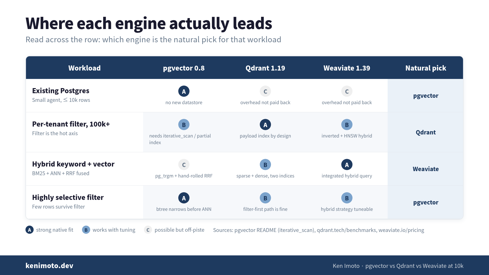
Prototype or small agent on existing Postgres: pgvector. My test says the filter cliff does not appear at 10k rows, and pgvector 0.8.0+ has iterative_scan waiting when it eventually does. Do not add a new datastore for four figures of vectors.
Production agent, per-tenant filtering, 100k+ vectors, no existing Postgres: Qdrant Cloud. Their benchmark exists to demonstrate they are best at this specific axis, and honestly, they are.
Multi-tenant hybrid keyword + vector search you actually rely on: Weaviate. Integrated BM25 + vector with reciprocal-rank fusion is worth the price step and it will save the code you were going to write to fuse two indexes yourself. pgvector needs pg_trgm and hand-rolled RRF; Qdrant needs sparse vectors and named indices.
You answer “which database” with “Postgres” to everything: keep doing that. Design the schema so common filters narrow fast — a btree on the filter column plus a partial HNSW index gives you the pgvector README’s recommended path. When the filter narrows fast, pgvector wins on the shape of the problem, and the same principle also underpins ChatGPT Codex vs Claude Code’s official-agent comparison: the datastore choice is downstream of how the query narrows.

I did not end up moving anything. My agent memory is 8,400 rows on managed Postgres, the “search across a project” queries return in single-digit milliseconds, and the day I cross six figures I will run the three-engine benchmark I was going to write today — at the scale where it actually separates them, not before.

Raw numbers and script

Two hundred queries per condition, pgvector 0.8.6, Postgres 17, HNSW m=16 ef_construction=64, single laptop, warm cache.

=== default HNSW (iterative_scan OFF) ===
  unfiltered top-10                                p50=1.31ms  p95=1.67ms  p99=1.88ms
  filter project_id (1/20 rows), post-filter       p50=1.88ms  p95=3.20ms  p99=3.48ms
  filter agent+time (near-empty), post-filter      p50=1.39ms  p95=2.53ms  p99=3.82ms

=== hnsw.iterative_scan = strict_order ===
  filter project_id (1/20 rows), iterative strict  p50=1.72ms  p95=2.42ms  p99=2.67ms

=== hnsw.iterative_scan = relaxed_order ===
  filter project_id (1/20 rows), iterative relaxed p50=1.67ms  p95=1.91ms  p99=2.09ms

Rows returned per query (want 10):
  default HNSW              : min=10 median=10 max=10  (across 30 samples)
  iterative_scan strict     : min=10 median=10 max=10  (across 30 samples)

The row-count check is the important one. If post-filter were breaking recall, some queries would come back with fewer than ten rows. None did. hnsw.ef_search=40 (the default) plus 500 candidates from a 1-in-20 filter is enough headroom that HNSW never starves. The moment the ratio flips — a million rows, or a tighter filter, or a lower ef_search — you will need iterative_scan or a partial index. Not before.

If retrieval, chunking, and where these decisions sit inside a full context stack are useful to you, that is chapter 6 of my Context Engineering book. The book measures the RAG side of the same question this post measures the storage side of.